Petr Frantík1, Volkmar Zabel2
This paper is especially created for studies in ESA interest groups.
Introduction
Theory of dynamical systems can be applied in investigation of complicated problems in structural mechanics, mainly in nonlinear dynamics. This theory gives possibility for wider view at solving problems, new methods for observing of a system evolution, the recognition of the general states of a system behaviour.
Here, some basic applications of this theory to the dynamic stability of a slender beam with large displacement are presented.
Static stability
The first step in understanding of a system's behaviour with respect to the theory of dynamical systems is the knowledge of its fixed points, if they exist. In structural mechanics is common to speak about statics (static states). All static solutions of the system are wanted fixed points.
Fig. 1 Beam buckling
Beam buckling is the fundamental problem of structural mechanics (see fig. 1). This problem is suitable for the demonstration of the influence of fixed points on a system's behaviour. If we have a perfect slender beam of linear elastic material with constant properties, then we can approximately derive the following equation3:
| (1) |
where  is the end rotation of the beam, F is the external force, Fcr is the critical value of force F, L is the length of the beam and EI is beam's bending stiffness. The solution of this equation can be written as:
 | (2) |
Solution one is trivial and precritical (stable only if force F is lower then the critical force Fcr, otherwise it is unstable). The next two stable solutions are postcritical and symmetric, i.e. they only exist if the force F is greater than the critical force Fcr (see fig. 2). A very good approximation of the maximal diagonal deflection y can be given by:
 | (3) |
However, a perfect beam is not real. We have always some imperfections (symmetry disturbance), which can be included in equation (1), for example:
 | (4) |
where imp is a geometric imperfection.
The perfect beam solutions (2) and the equivalent solutions of the imperfect problem (4) are illustrated in fig. 2.
Fig. 2 Graph of static solutions
In fig. 2 we can see the development of the static solutions with respect to the force F and influence of an imperfection. First we have only one solution ( F < Fcr) - precritical zone. The solution is bifurcated for F > Fcr (postcritical zone) to two symmetric (similar) solutions.
SDOF model4
For fast dynamic calculations and a first introduction into special tools used in the theory of dynamical systems it is suitable to consider a single-degree-of-freedom (SDOF) model. A possible dynamic SDOF model for beam buckling is shown in fig. 3.
The beam is modelled by two rigid elements that are connected by a hinge with linear rotational spring. The mass M is concentrated at the hinge. The moment m at the spring is:
 | (5) |
where k is the stiffness of the spring.
Fig. 3 SDOF model
The model (without time dependent load) has two state variables (unknown time series, which we want to calculate): rotation and angle velocity  . The angle velocity is defined:
 | (6) |
The beam is loaded by gravity g and by a harmonic force P:
 | (7) |
where A is the amplitude of the force,  is the circular frequency of the force and t is the time.
The model can be described a system of differential equations [3]:
 | (8) |
where  is phase angle of the harmonic force P (third state variable). For the phase angle we have = t. And c is a linear damping coefficient (i.e. we have a system with energy dissipation).
The solution of the system of equations (8) can be found by means of any numerical method, e.g. the simple Euler method or the Runge-Kutt method.
Example 1: Solution of the system equations by means of the Euler method
The application of the Euler method to the system (8) is straight forward. The system (8) can be formulated more generally:
 | (9) |
where  ,
,  ,
,  are known initial conditions of the system. We can choose any time step h and calculate an approximation of the system's state at time t = h:
 | (10) |
generally in time t becomes:
 | (11) |
The precision of the numerical results mainly depends on the time step h. We must check the stability of calculation and compare results with other results (obtained from using different time step h or another numerical method).
Visualisation
Special visualisation tools are used in theory of dynamical systems. It is given by the general properties of the problem. This is necessary in strong nonlinear dynamics, because we can obtain a very complicated behaviour.
The solution of the dynamical systems is best described in phase space. The phase space is a "virtual" space, where the system's state variables are space dimensions. Our SDOF model, described by system (8), has three state variables. According to this, the phase space has three dimensions, see fig. 4.
Fig. 4 Phase space
Each point in phase space completely determines the system's state and its development. The development of the system is represented in phase space by a continuous curve the so-called trajectory of the system.
Example 2: Visualisation in phase space
We can demonstrate the properties of the defined visualisation tools by a free vibration of a simple damped linear model in a two-dimensional phase space. On the right side in the fig. 5 is a time series of free oscillations of a linear damped model. On the left side the same time series is given in phase space. We can see a fixed point like an attractor in the phase space.
Fig. 5 Visualisation of a simple trajectory; left: projection in phase space (displacement and its velocity), right: time series of displacement
Example 2 has a two-dimensional phase space (fig. 5). There is a problem with phase space visualisation, if we have a more-dimensional system (like our SDOF beam buckling model). We can use a phase space projection for the visualisation of a more-dimensional system's development. For example: The trajectory on the left side in figure 6 is three-dimensional and we can project it to the plane , see right side in fig. 6.
Fig. 6 Three-dimensional trajectory and its projection
But every projection has wrong properties, because some information gets lost.
Example 3: Steady state
This example is about the visualisation of the steady state of a linear harmonically loaded system (for example a simple spring or our beam buckling model only with small displacements). Such a system can be three-dimensional and we know, that the steady state of this system is also a harmonic motion. This steady state is the simplest so-called limit cycle. The projection of this limit cycle (to displacement-velocity plane) is shown on left side in fig. 7. The time series of the displacements is illustrated on the right.
A harmonic motion is a spiral in the phase space. Its projection is an ellipse (circle). A change of the form of the elliptic limit cycle into something, that is different from ellipse, is good indicator for a nonlinearity in tested system.
Fig. 7 Limit cycle projection and displacement time series
Bifurcation
Nonlinear dynamical systems have something, what is fundamentally different from anything, that we can find for linear systems. This is the bifurcation of the limit cycle. We can obtain a bifurcation due to change of the parameters of a system. For some set of a parameters we have a simple limit cycle (for example on left side in fig. 8). This simple limit cycle has any period. Due to a small change of one parameter we can obtain a bifurcated limit cycle with a double period (like on right side in fig. 8).
Fig. 8 Limit cycle bifurcation
Every limit cycle (also bifurcated limit cycles) can bifurcate again and again. This process is called period-doubling and looks like a cascade of bifurcations. We need a new tool for the visualisation of this process, the so-called Poincare map. The Poincare map is something like a cut of trajectory. For our system (8) we can define the Poincare map by a set of all points on system trajectory for which apply:
 | (12) |
Example 4: Poincare map
We can see applicability of the defined Poincare map to the simple and bifurcated limit cycle shown in fig. 8. The simple limit cycle has only one point in the Poincare map (every points has the same position) and the bifurcated limit cycle has two points (every point is either at the first position or at the second position), see fig. 9.
Fig. 9 Points in Poincare map
Dependency of a Poincare map can be shown due to slow change of parameter. We can select one state variable (for example in our SDOF model (8)) and calculate the whole process of bifurcation and show it in the bifurcation diagram. In fig. 10 an example of a simple bifurcation diagram with "cascade of bifurcation" is illustrated.
Fig. 10 Illustration of a simple bifurcation diagram
After a period-doubling we can obtain chaotic behaviour, which is situated behind converged "cascade of bifurcation". Chaotic behaviour is a non-periodic motion and often close doubling of limit cycles.
Example 5: Chaos in SDOF model of beam buckling
We can show results from a simulation of our system (8), which is a SDOF model of beam buckling. In fig. 11 some steady states of this model are illustrated. Parameters are: g =9.81 m.s-2, c =0.1 N.s.m-1, m =0.21 kg, L =0.723 m, k =0.3921 N.m.rad-1, imp =0.005 rad, =2 rad.s-1 and amplitude A = 0.3 … 0.35 N. In fig. 11 the first two bifurcations of the limit cycle are shown and in fig. 12 chaotic attractor and its Poincare map are given.
Fig. 11 Period-doubling in SDOF model of beam buckling
Fig. 12 Chaotic attractor and its Poincare map
Special model of cantilever beam5
For experimental research a special model of a cantilever beam was created. A similar discretization as for the SDOF model of beam buckling was applied. The beam is divided into a number of rigid elements connected by hinges with linear rotational springs, see fig. 13.
Fig. 13 Slender cantilever beam and its special model
It is possible to say, that this model is only an expansion of the described SDOF model. The static solution and the free vibration of this model agree very well with the experimental results. A verification (in dynamic stability problems) of this model is in progress now.
Experimental setup
The experimental setup for the models verification is illustrated in fig. 14. There is a hydraulic cylinder with a moving piston, which moves up and down in vertical direction. On the piston the tested slender beam with an additional mass at the free end was mounted. The beam is in static postcritical state. The displacement of the piston is harmonic (controlled by a computer attached to hydraulic machine).
Fig. 14 experimental setup
Experimental setup
The general theory of relativity gives us the theorem of absolute equality between the effects of acceleration and gravity. With respect to this theorem, we can describe the acceleration at the beam's base (fixation on the piston) as a change of the gravity field. This is main idea of the representation of the beam's base motion in the model.
Example 6: Conversion of amplitudes
If we have a harmonic motion (like motion of the piston) we can convert displacements to accelerations. Let's consider any position of any point x(t), which is given by:
 | (13) |
where Amot is the amplitude of the point displacement and is the circular frequency. Then we can derive the acceleration of the point x(t):
 | (14) |
where Aaccel is amplitude of the point's acceleration.
Numerical results
In a previous part was described, that we need to obtain nonlinear behaviour for a strong verification of the model. If we want large displacements with small strains (elastic behaviour), we have to use a slender beam of a suitable material and suitable parameters. Our tested beam has these parameters:
The load (due to piston's motion) has these parameters:
= 3.1416 rad.s-1 (frequency  = 0.5 Hz),
We will start every simulation and experiment from the static state (postcritical state) on the side of the imperfection.
Example 7: Simple 1-point limit cycle (Aaccel = 0.2 m.s-2)
In fig. 15 we can see the GUI (Graphic User Interface) of the Java simulation applet for the special cantilever beam model. In the top are the inputs of important values like the number of elements, the time step, the initial conditions. In the bottom are the inputs of parameters. In the centre of the window is system development plot: At the left is the animation of the beam's motion, in the middle of this part is the projection of system's trajectory to the plane Y Y , where Y is the diagonal displacement of beam's free end and at the right is the Poincare map.
We can see, that the system has a simple limit cycle with one point in Poincare map for an acceleration amplitude Aaccel =0.2 m.s-2 ( Aamp x in applet - applet is more general).
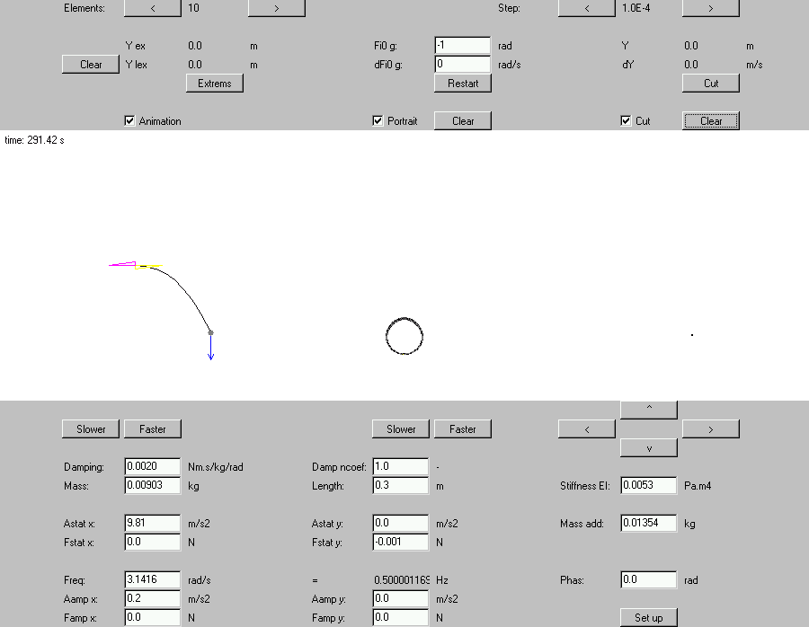
Fig. 15 Applet GUI with 1-point limit cycle
Example 8: 2-point limit cycle (Aaccel = 0.6 m.s-2)
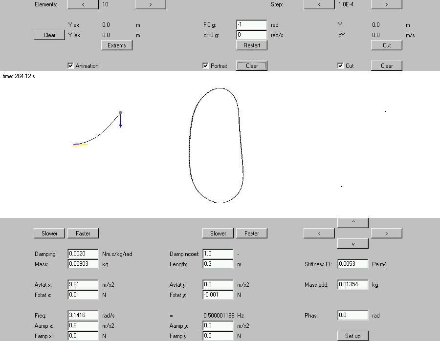
Fig. 16 Applet GUI with 2-point limit cycle
Example 9: 3-point limit cycle (Aaccel = 0.69 m.s-2)
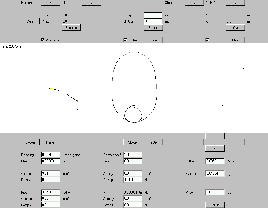
Fig. 17 Applet GUI with 3-point limit cycle
Example 10: chaotic attractor (Aaccel = 0.9 m.s-2)
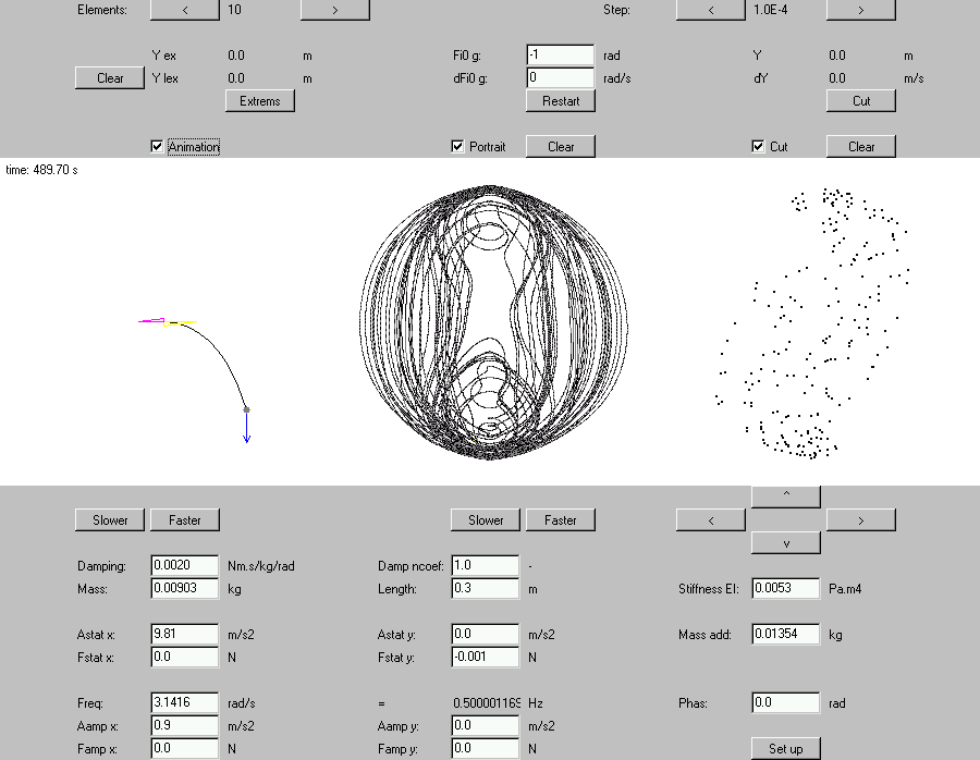
Fig. 18 Applet GUI with chaotic attractor
Example 11: Bifurcation diagram
In fig. 19 is shown a bifurcation diagram with respect to the parameter Aaccel (amplitude of acceleration). For 400 separate simulations (steadying time 300 seconds) 50 points were drawn in Poincare map. We can see an undisturbed part with a 1-point limit cycle, then a by chaos disturbed part with a 2-point limit cycle, followed by a part with a 3-point limit cycle and finally the chaos part.
Fig. 19 Bifurcation diagram
Acknowledgements
The Authors wish to thank Prof. Christian Bucher and Prof. Drahomír Novák for the possibility of experimental research at the Bauhaus University Weimar.
The funding under project Socrates-Erasmus, the Czech Republic research project reg. No. CEZ: J22/98: 261100009 and grant No. 103/03/1350 from the Grant Agency of the Czech Republic are gratefully acknowledged.
Note
For this paper materials from many papers, mainly in czech language were used, which are available on http://kitnarf.cz/.
1Brno University of Technology, Czech Republic, e-mail: kitnarf at centrum.cz
2Bauhaus University Weimar, Germany, e-mail: volkmar.zabel at bauing.uni-weimar.de
3This equation is obtained from single-degree-of-freedom model of beam buckling
4Java simulation of this model is available on http://www.fce.vutbr.cz/STM/frantik.p/applets/vzper/simul.htm
5Equations of motion are available on http://kitnarf.webpark.cz/2003.05.dynwind/2003.05.dynwind.htm, but in this time only in czech language